Andrey SERY*
Commissariat à l'Energie Atomique, DSM/DAPNIA
Saclay, F-91191 Gif-sur-Yvette Cedex, France
The future TeV linear collider should have extremely small beam emittance to achieve the required luminosity. Precise alignment of focusing and accelerating elements is necessary to prevent emittance dilution. Analysis of ground motion is therefore an essential problem.
This paper reviews studies of ground motion, focusing on the effects the in main linac. After recalling results of measurements of ground motion collected at different places, the method based on spectral description of ground motion, which allows prediction of emittance dilution, in presence of orbit correction feedback as well, is discussed.
The first study of ground motion with respect to linear collider was performed at SLAC by G. Fischer [1]. The intention to build TeV linear collider has inspired new studies started at Protvino [2] and since then in all laboratories developing linear collider projects [3]-[7].
The level of understanding of ground motion has been developed significantly in recent years. The correlation properties of high frequency motion have been investigated [2, 3, 7] in addition to simple spectral amplitude analysis. The slow motion investigations have resulted in discovering of the diffusive ground motion (``ATL law'' [2]). Dependance of motion on the earth structure was studied [12, 6].
The mathematics, which allows prediction of the effect on
the beam, was also being developed in parallel to measurements.
The 2-D power spectrum ![]() ,
introduced for ground motion description [4, 8],
makes the evaluation of the effect on the beam easy and natural --
once this spectrum,
the spectral response function of the
focusing structure and the spectral properties
of applied orbit correction feedbacks are known.
The measured data were used to to find
an approximation of
,
introduced for ground motion description [4, 8],
makes the evaluation of the effect on the beam easy and natural --
once this spectrum,
the spectral response function of the
focusing structure and the spectral properties
of applied orbit correction feedbacks are known.
The measured data were used to to find
an approximation of ![]() [8]
for typical seismic conditions.
[8]
for typical seismic conditions.
This paper intends to show the complete way from measurements to the beam emittance growth. We start from general equations, then consider measured data, create approximation of the 2-D spectrum, and get results using spectral response functions and feedback properties. The misalignment generated beam offset and dispersion in the main regular linac governed by the ``one to one'' orbit correction is used to illustrate our considerations.
Misalignments of focusing quadrupoles of the linac produce offset of the beam trajectory and hence chromatic dilution of the beam, which can be expressed via an integral involving the power spectrum of the quadrupole displacements and a spectral response function of the considered linac.
Let ![]() be the transverse position
of quadrupoles of the linac, relatively to a reference line,
be the transverse position
of quadrupoles of the linac, relatively to a reference line,
![]() the longitudinal position.
The incoming beam angle and position are zero, the reference
line passes through some element, placed at the entrance.
The beam offset at the exit, relative to the exit position
the longitudinal position.
The incoming beam angle and position are zero, the reference
line passes through some element, placed at the entrance.
The beam offset at the exit, relative to the exit position
![]() ,
and the dispersion, linear term, are
,
and the dispersion, linear term, are
![]()
Here ![]() and
and ![]() are the first derivatives of the beam
offset and dispersion at the exit of the linac with respect
to the displacement of the i-th quadrupole.
are the first derivatives of the beam
offset and dispersion at the exit of the linac with respect
to the displacement of the i-th quadrupole.
While ![]() and
and ![]() ,
averaged on realizations, are zero,
the mean squared value gives the offset or dispersive error,
for example
,
averaged on realizations, are zero,
the mean squared value gives the offset or dispersive error,
for example
![]()
As we consider random process, one can
express this through the corresponding power
spectrum P(t,k).
For initial misalignment or (and) ground motion
all spatial harmonics are independent. We have then
![]()
Here ![]() is the so called spectral response function
corresponding to dispersion. The expression for the offset
is similar, with
is the so called spectral response function
corresponding to dispersion. The expression for the offset
is similar, with ![]() .
The expression allows to obtain results for any spectrum,
including the particular case of static gaussian
misalignments studied in detail [9].
.
The expression allows to obtain results for any spectrum,
including the particular case of static gaussian
misalignments studied in detail [9].
The spatial power spectrum P(t , k) of displacements x(t,s)
can be easily found as far as initial misalignment or ground motion
are concerned.
Assuming that focusing elements are aligned
at t=0 and then are moved by ground motion,
the evolution of the power spectrum is [4]:
![]()
It is connected therefore to the 2-D power spectrum
![]() , which characterizes ground motion properties,
including both spatial and temporal correlation information.
, which characterizes ground motion properties,
including both spatial and temporal correlation information.
In a regular linac the correction procedures can also
be correctly considered within the analytical spectral approach.
Correction procedures, such as ``one to one'' or ``adaptive alignment''
[10] may introduce correlation of phases
between harmonics
k and ![]() (where
(where ![]() , L is the quadrupole spacing).
The rms dispersion is then given by an expression,
which takes the correlation into account [14].
, L is the quadrupole spacing).
The rms dispersion is then given by an expression,
which takes the correlation into account [14].
In short, the spectral response functions G (k) describe the properties of the focusing channel, while the power spectrum P(t,k) depends on the applied method of correction, initial misalignment and ground motion.
The 2-D spectrum ![]() is hard to measure directly.
But if one knows the power spectra of absolute motion
and correlation information, or the power spectra of relative
motion
is hard to measure directly.
But if one knows the power spectra of absolute motion
and correlation information, or the power spectra of relative
motion ![]() , the 2-D spectrum can be found using
, the 2-D spectrum can be found using
![]()
and the reverse relation [4].
Naturally, ![]() .
The measurable correlation, defined via mutual spectrum as
.
The measurable correlation, defined via mutual spectrum as
![]() , connected to the relative
spectrum as
, connected to the relative
spectrum as ![]() .
.
The power spectrum ![]() of absolute ground motion
(which contains contribution of all k)
grows very fast with decreasing
frequency. In quiet conditions it behaves approximately as
of absolute ground motion
(which contains contribution of all k)
grows very fast with decreasing
frequency. In quiet conditions it behaves approximately as
![]() in rather wide frequency band.
The motion is unavoidable as it consists of seismic
activity. At low frequency f < 1 Hz the sources
are also the atmospheric activity, water motion in the
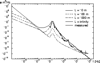
oceans, temperature variations etc. A famous example of the ocean
influence is the peak in the band
0.1 - 0.2 Hz with a few micrometers amplitude (Fig.1).
In general, motion in the low
frequency band f < 1 Hz depend not only on the
local conditions, remote sources give significant
contribution to the slow motion.
in rather wide frequency band.
The motion is unavoidable as it consists of seismic
activity. At low frequency f < 1 Hz the sources
are also the atmospheric activity, water motion in the
oceans, temperature variations etc. A famous example of the ocean
influence is the peak in the band
0.1 - 0.2 Hz with a few micrometers amplitude (Fig.1).
In general, motion in the low
frequency band f < 1 Hz depend not only on the
local conditions, remote sources give significant
contribution to the slow motion.
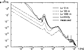
From the other side, in the band f > 1 Hz the human produced noises are usually dominating over the natural noises and the power spectrum depends very much on the local conditions (location of sources, depth of tunnel etc.). Locally generated noises can be much bigger than remotely generated. For example the spectrum measured at the tunnel of operating accelerator (like HERA collider at DESY or SLC at SLAC) presents high amplitudes at f > 1 Hz due to noises generated by different technical devices (Fig.2). These noises may have big amplitude and bad correlation. Technical devices therefore should be properly designed in order to pass as low vibration as possible to the tunnel floor.
It is known from correlation measurements [3, 7] that in quiet
conditions the motion in the band f > 0.1 Hz can be considered
as wave-like, i.e. the frequency ![]() and wave number k
are connected via phase velocity v. At
and wave number k
are connected via phase velocity v. At ![]() Hz the
value of v was found to be close to the velocity of sound
(in the surrounding media): about 3000 m/s at LEP and
about 2000 m/s at SLC tunnel. At the cultural noise dominated
band this value decreases rapidly -- the fitted value of v determined
from the measured at SLAC correlation behave as
Hz the
value of v was found to be close to the velocity of sound
(in the surrounding media): about 3000 m/s at LEP and
about 2000 m/s at SLC tunnel. At the cultural noise dominated
band this value decreases rapidly -- the fitted value of v determined
from the measured at SLAC correlation behave as
![]() m/s (f > 0.1 Hz) [7].
The SLAC measurements, which used the most accurate probes,
have shown (at least at this place and these conditions)
that contribution of non-wave motion, if there is any
not resolved by probes, is negligible at f>0.1 Hz.
m/s (f > 0.1 Hz) [7].
The SLAC measurements, which used the most accurate probes,
have shown (at least at this place and these conditions)
that contribution of non-wave motion, if there is any
not resolved by probes, is negligible at f>0.1 Hz.
The motion at f < 0.1 Hz is different.
The elastic motion (produced by the moon, for example)
presents here too, but of much bigger relevance is the inelastic
diffusive motion, probably fed by the elastic motion and
caused by its dissipation. The motion is
believed to be described by the ``ATL law'' [2],
which says that the relative rms displacement after a time T of
the two points separated by a distance L is
![]() .
The parameter A was found to be
.
The parameter A was found to be
![]()
![]() m
m ![]() s
s ![]() m
m ![]() for different places.
One can see that this displacement is proportional
to the square root of the time and separation:
this stresses the random, non
wavelike, diffusion character of the slow relative
motion and means
that the number of step-like breaks
that appear between two points is proportional to the
distance between them and the elapsed time.
for different places.
One can see that this displacement is proportional
to the square root of the time and separation:
this stresses the random, non
wavelike, diffusion character of the slow relative
motion and means
that the number of step-like breaks
that appear between two points is proportional to the
distance between them and the elapsed time.
If this phenomenon is indeed connected with dissipation of
the elastic motion, the parameter A should depend mainly
on the earth properties, because the sources of elastic motion are the
same for all places.
One could expect that in the places
with smaller dissipation the
value A should be smaller and it should also depend on
the level of the rock fragmentation.
Indeed, the parameter A was observed to
be smaller in tunnels built in solid rock.
It also depends on the method of tunnel construction:
in the tunnel bored
in granite ![]()
![]() m
m ![]() s
s ![]() m
m ![]() was observed, while
in the similar tunnel, which was built by use of explosions,
the parameter A is found to be 5 times larger probably
because of the fragmentation, artificially increased during
construction [6]. The parameter A also depends on the
tunnel depth, generally it is smaller in deeper tunnels [12].
was observed, while
in the similar tunnel, which was built by use of explosions,
the parameter A is found to be 5 times larger probably
because of the fragmentation, artificially increased during
construction [6]. The parameter A also depends on the
tunnel depth, generally it is smaller in deeper tunnels [12].
The ranges of T and L where the ``ATL law'' is valid
are very wide. In [12] it was summarized that ``ATL''
is confirmed by
measurements of ground motion in different accelerator tunnels
in the range from minutes to tens of years and from a few meters
to tens of kilometers. The measured relative power spectra, presented
in [6] and in [11], exhibit the ``ATL''
behavior already for f < 0.1 Hz (for ![]() m).
These measurements indicate that the transition region
from wave to diffusion motion is placed at rather
short times (a few seconds). This can result in certain decreasing
of correlation around
m).
These measurements indicate that the transition region
from wave to diffusion motion is placed at rather
short times (a few seconds). This can result in certain decreasing
of correlation around ![]() Hz.
Hz.
Although the ``ATL law'' was found from the direct analysis of
measurements of ground motion, its most interesting
confirmations come from the observations of beam
motion in big accelerators
produced by displacements of the focusing elements.
An example is the measurements of the closed orbit motion
in the HERA circular collider, which have shown
that the power spectrum
of this motion corresponds to the ``ATL law'' in a wide
frequency range, from ![]() Hz
down to
Hz
down to ![]() Hz [11].
Hz [11].
The very slow motion can be systematic (not described by power spectrum) as well. Such motion has been observed at LEP Point 1 and PEP [13] where some quadrupoles move unidirectionally during many years with rate about 0.1 - 1 mm/year. Quite close (a few tens of meters) points can move in opposite direction. Amplitude of the motion can be larger than the one of diffusive motion. The motion is probably due to geological peculiarities of the place or due to relaxation if the tunnel was bored in solid rock.
Ending with the ground motion one could note that the elements of the linac will be placed not on the floor, but on some girder, which could amplify some frequencies due to its own resonances. It is not only this amplification that is dangerous, more important is that the not identical girders will amplify or change the floor motion by different way, which can spoil correlation of the floor motion. It is therefore preferable to push the girder resonances to high frequencies where the correlation is poor anyway and floor amplitudes are smaller. This requires firm connection of the girder with the floor. The active systems [15], which can help in certain extend to isolate the quadrupoles from high frequency human induced floor motion, should be made insensitive to slow motion (say, below 1 Hz), otherwise long wavelength motion can create more dangerous short wavelength due to inequality of active supports.
The approximation for ![]() is built [8] in
assumption that the low frequency part of motion is
described by the ``ATL law'', while the high frequency part
is produced mainly by waves. The 2-D spectrum corresponded
the ``ATL'' motion is
is built [8] in
assumption that the low frequency part of motion is
described by the ``ATL law'', while the high frequency part
is produced mainly by waves. The 2-D spectrum corresponded
the ``ATL'' motion is ![]() (here
(here ![]() and k are defined on the entire axis). In order to be
included into the model, this spectrum should be corrected
because it overestimates fast motion -- the corresponded
spectrum of relative motion exceeds the one of absolute motion.
The correction is made by the way that will overestimate the effect
rather than underestimate it. Better model can be built once
measured data on transition region are available.
The elastic waves are assumed to be transverse, propagating at
the surface of the ground with uniform distribution
over azimuthal angle.
Finally, the modeling spectrum is:
and k are defined on the entire axis). In order to be
included into the model, this spectrum should be corrected
because it overestimates fast motion -- the corresponded
spectrum of relative motion exceeds the one of absolute motion.
The correction is made by the way that will overestimate the effect
rather than underestimate it. Better model can be built once
measured data on transition region are available.
The elastic waves are assumed to be transverse, propagating at
the surface of the ground with uniform distribution
over azimuthal angle.
Finally, the modeling spectrum is:
![]()
The function ![]() describes the wave number
distribution
of the waves with frequency
describes the wave number
distribution
of the waves with frequency ![]() . In our case
. In our case
![]() if
if ![]() and zero otherwise.
Here
and zero otherwise.
Here ![]() and
and
![]() the phase velocity of wave propagation.
The cases k=0 and
the phase velocity of wave propagation.
The cases k=0 and ![]() correspond to the waves
propagating perpendicular and along the linear collider
correspondingly.
Since the integral over
correspond to the waves
propagating perpendicular and along the linear collider
correspondingly.
Since the integral over ![]() of
of ![]() equals one, the function
equals one, the function ![]() describes contribution
of these waves to the absolute spectrum
describes contribution
of these waves to the absolute spectrum ![]() .
We write
.
We write ![]() as
as
![]() .
In order to model complex behavior of the spectrum, for
example in presence of cultural noises, a few terms with waves
added to
.
In order to model complex behavior of the spectrum, for
example in presence of cultural noises, a few terms with waves
added to ![]() , i is the number of the peak.
, i is the number of the peak.
We consider here two models. Parameters of the first model
are the following: ![]()
![]() m
m ![]() s
s ![]() m
m ![]() ,
,
![]()
![]() m
m ![]() s
s ![]() .
The single peak described by
.
The single peak described by
![]() Hz for the frequency of the peak,
Hz for the frequency of the peak,
![]() m
m ![]() /Hz for its amplitude,
/Hz for its amplitude,
![]() for its width, and
for its width, and
![]() m/s for the velocity.
It is the model of quiet place such as LEP tunnel during shutdown.
The thick line on Fig.1 shows
the spectrum of absolute motion, calculated from
m/s for the velocity.
It is the model of quiet place such as LEP tunnel during shutdown.
The thick line on Fig.1 shows
the spectrum of absolute motion, calculated from ![]() ,
corresponding to these parameters.
The actual measured
,
corresponding to these parameters.
The actual measured ![]() can be bigger than the modeling
one at f<0.1 Hz,
because slow long wavelength motion does not included into
the model.
The second model corresponds to seismic conditions
with big contributions
from cultural noises (as in the HERA tunnel in operating conditions).
The parameters are the following:
can be bigger than the modeling
one at f<0.1 Hz,
because slow long wavelength motion does not included into
the model.
The second model corresponds to seismic conditions
with big contributions
from cultural noises (as in the HERA tunnel in operating conditions).
The parameters are the following:
![]()
![]() m
m ![]() s
s ![]() m
m ![]() ,
,
![]()
![]() m
m ![]() s
s ![]() and
three peaks:
and
three peaks:
![]() ,
, ![]() ,
, ![]() Hz;
Hz;
![]() ,
, ![]() ,
, ![]() m
m ![]() /Hz;
/Hz;
![]() ,
, ![]() ,
, ![]() ;
;
![]() ,
, ![]() ,
, ![]() m/s.
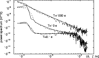
One can see (Fig.3) how the waves are faded by the ``ATL''
in P(t,k) when time increases.
The parameters of these two models have been chosen taking
into account correlation measurements in the LEP [3], HERA
[5] and SLC [7] tunnels and
measurements of the closed orbit
motion in HERA [11].
m/s.
One can see (Fig.3) how the waves are faded by the ``ATL''
in P(t,k) when time increases.
The parameters of these two models have been chosen taking
into account correlation measurements in the LEP [3], HERA
[5] and SLC [7] tunnels and
measurements of the closed orbit
motion in HERA [11].
The effect of the ground motion on the beam can be obtained
both by analytical
way via the integral of spectral function with the
modeling power spectrum
and also by simulations, when ground motion
displacement x(t,s) is modelized by summation of harmonics
and the beam degradation determined by particle tracking.
In the latter case we first analyze the modeling
![]() spectrum to define
the band of relevant
spectrum to define
the band of relevant ![]() and k, assuming
that
and k, assuming
that ![]() and
and
![]() .
Then we split this 2-D band by cells
(
.
Then we split this 2-D band by cells
( ![]() typically) equidistantly in logarithmic sense,
find rms amplitude of each cell
typically) equidistantly in logarithmic sense,
find rms amplitude of each cell ![]() and generate two sets of random
phases
and generate two sets of random
phases ![]() and
and ![]() . Positions of
. Positions of ![]() and
and ![]() withing each cells are chosen randomly so
after many seeds all
withing each cells are chosen randomly so
after many seeds all ![]() will be checked.
The modeling displacement x(t,s) is then
will be checked.
The modeling displacement x(t,s) is then
![]()
![]()
This harmonics model was used in our simulations, eventually
it will be used in the linear collider flight simulator
``MERLIN'' [16], which is
being developed to analyze performance of the beam delivery systems.
The spectral response function corresponded to
dispersion of the beam is
Similar for the offset, with ![]() , with the sum runs
up to N+1 and
, with the sum runs
up to N+1 and ![]() .
In thin lens approximation, in
linear order
.
In thin lens approximation, in
linear order ![]() and
and
![]() where
where ![]() is
is ![]() of the quadrupole matrix,
of the quadrupole matrix,
![]() and
and ![]() are the matrix elements
from the i-th quadrupole to the exit.
are the matrix elements
from the i-th quadrupole to the exit.
At small k one has ![]() and
and ![]() .
For the regular linac only the band
.
For the regular linac only the band ![]() is unique.
In this band the spectral function has two resonances:
is unique.
In this band the spectral function has two resonances:
![]() and
and ![]() .
The values of spectral function at these resonances
as well as their width can be found analytically.
.
The values of spectral function at these resonances
as well as their width can be found analytically.
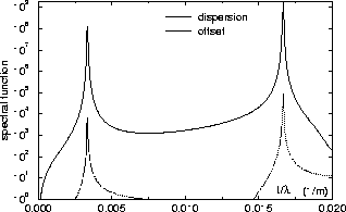
The examples in this paper are given for the modeling FODO linac:
number of quadrupoles N=600, spacing L=25 m,
phase advance ![]() degrees,
initial and final energy
degrees,
initial and final energy ![]() ,
,
![]() ,
beta functions at the even defocusing quadrupoles and at
the exit are
,
beta functions at the even defocusing quadrupoles and at
the exit are ![]() m.
The spectral functions for this linac are shown on Fig.4.
m.
The spectral functions for this linac are shown on Fig.4.
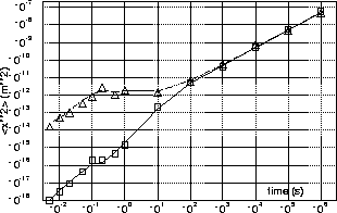
Fig.5 shows the rms beam offset relative
to the linac exit versus time for quiet and noisy models
of ground motion.
The analytical results are shown in comparing
with results of simulations, which use tracking and the
model of harmonics to simulate beam line misalignment.
To estimate the critical time scale, this offset should be
compared with the beam size at the exit.
If ![]() m, then at the
exit
m, then at the
exit ![]() m and the
critical time is about one minute. For somewhat smaller
emittance the cultural noise of the second model
becomes important and the critical time decreases
to a fraction of second.
m and the
critical time is about one minute. For somewhat smaller
emittance the cultural noise of the second model
becomes important and the critical time decreases
to a fraction of second.
One can see that the chosen
![]() spectrum gives a linear dependence
of the relative misalignment variance
(and hence the rms beam offset as well)
versus time for large T
(``ATL'' behavior), while for small T the
variance is proportional to
spectrum gives a linear dependence
of the relative misalignment variance
(and hence the rms beam offset as well)
versus time for large T
(``ATL'' behavior), while for small T the
variance is proportional to ![]() .
This square dependence at small time
is the general property of the spectrum that drops fast enough
with increasing frequency [17].
One can mention that if the systematic motion is
significant, the
.
This square dependence at small time
is the general property of the spectrum that drops fast enough
with increasing frequency [17].
One can mention that if the systematic motion is
significant, the ![]() behavior will appear at
big T too.
behavior will appear at
big T too.
Many feedbacks will inevitably be used in linear collider.
To study the equilibrium
rms offset accurately, one need to put the feedback gain function
into the integral, which will suppress frequencies
smaller than ![]() -
- ![]() .
.
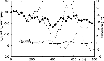
To illustrate influence of an orbit correction feedback on the beam dispersion, let us consider the ``one-to-one'' algorithm, which consists in zeroing the BPM measurements (assumed to be perfect). Here we assume that this is done by steering the beam by means of dipole correctors (equivalent to the quadrupole shift). This and other orbit correction or alignment methods are considered in more details (including BPM errors etc.) elsewhere [14].
If the i-th quadrupole is misaligned, three
angles are needed to re-align the beam. The
equivalent quadrupole displacements, to be subtracted
from their initial positions, are (if acceleration is neglected):
![]()
After such a procedure the beam trajectory will pass
through positions of quadrupoles before correction
(Fig.6).
To find the beam dispersion one can notice that
in spectral approach, in a regular FODO lattice with ![]() ,
a k-th harmonics of the initial misalignment
produces two harmonics of
quadrupole displacements after the correction:
k-th and
,
a k-th harmonics of the initial misalignment
produces two harmonics of
quadrupole displacements after the correction:
k-th and ![]() -th with opposite phases.
If this self correlation as well as injection conditions
are taken into account, the dispersion after correction
can be found [14].
-th with opposite phases.
If this self correlation as well as injection conditions
are taken into account, the dispersion after correction
can be found [14].
An alternative way to write the beam dispersion
after ``one-to-one'' correction is
where ![]() and
and ![]() are
the effective spectral response function and the
effective spectrum of quadrupole displacements
before correction (which can include BPM offset and resolution
errors also) respectively. The
are
the effective spectral response function and the
effective spectrum of quadrupole displacements
before correction (which can include BPM offset and resolution
errors also) respectively. The ![]() is built with new
coefficients (neglecting acceleration) [14]:
is built with new
coefficients (neglecting acceleration) [14]:
![]()
It gives ![]() .
This follows from the algorithm of correction --
the angle caused by displaced quadrupole
is corrected, thus the term
.
This follows from the algorithm of correction --
the angle caused by displaced quadrupole
is corrected, thus the term ![]() vanishes.
The
vanishes.
The ![]() and
and ![]() are practically the same
therefore.
are practically the same
therefore.
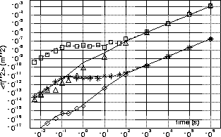
The considered ``one-to-one'' scheme reduce emittance
growth by factor ![]() roughly, which increase
significantly the time interval until a beam based
alignment might be again required. The critical time
(when
roughly, which increase
significantly the time interval until a beam based
alignment might be again required. The critical time
(when ![]() )
for the beam with
)
for the beam with ![]() is
a few hours without and about one year with
correction (Fig.7).
is
a few hours without and about one year with
correction (Fig.7).
Fig.7 shows dispersion without and with ``one-to-one'' correction. In the second case the dispersion is shown at the moment just after correction. This value does not depend on how many times the correction has been applied before. If the repetition rate of corrections is enough high, the values just after and just before correction are very close.
A future TeV linear collider, having extremely small emittance of beams, will suffer from the ground motion, which will spoil alignment of focusing and accelerating elements and result in offset and emittance growth.
The ground motion studies, performed by different laboratories, resulted in significant improvement of understanding of this phenomenon. Different types of motion have been investigated, many factors that the motion depends on are learned. The mathematical formalism allowing prediction of the beam behavior is developed.
Though many ground motion features are still to be carefully investigated, one may reasonably believe that the ground motion problem of the future linear collider can be overcame provided that stored knowledge will be used at each step of design and construction.
I am grateful to colleagues from Novosibirsk INP and Protvino Branch INP for being working together over many years and to colleagues from CERN, DESY, CEA Saclay and SEFT for fruitful collaborations. I am indebted to colleagues from KEK and SLAC for numerous helpful discussions.